
Supervised Learning
- Supervised learning is used whenever we want to predict a certain outcome from a given input, and we have examples of input/output pairs.
- Our goal is to make accurate predictions for new, never-before-seen data. Supervised learning often requires human effort to build the training set, but afterward automates and often speeds up an otherwise laborious or infeasible task.
- There are two major types of supervised machine learning problems, called classification and regression.
Content
- Classification and Regression
- Generalization, Overfitting, and Underfitting
- Relation of Model Complexity to Dataset Size
Supervised Machine Learning Algorithms
- Some Sample Datasets
- k-Nearest Neighbors
- Linear Models
- Naive Bayes Classifiers
- Decision Trees
- Ensembles of Decision Trees
- Kernelized Support Vector Machines
- Neural Networks (Deep Learning)
Uncertainty Estimates from Classifiers
- The Decision Function
- Predicting Probabilities
- Uncertainty in Multiclass Classification
- Summary and Outlook
1. Classification and Regression
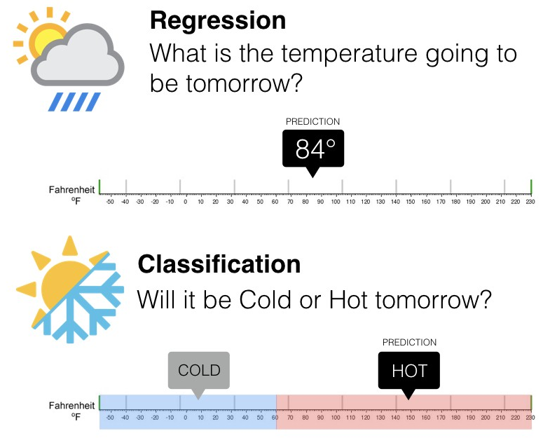
1.1 Classification
- The goal is to predict a class label, which is a choice from a predefined list of possibilities.
- Classification:
- Binary classification,which is the special case of distinguishing between exactly two classes
- Multiclass classification, which is classification between more than two classes.
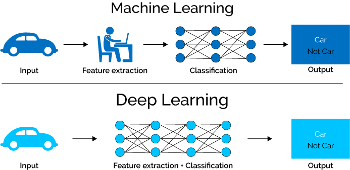
1.2 Regression
- The goal is to predict a continuous number, or a floating-point number in programming terms
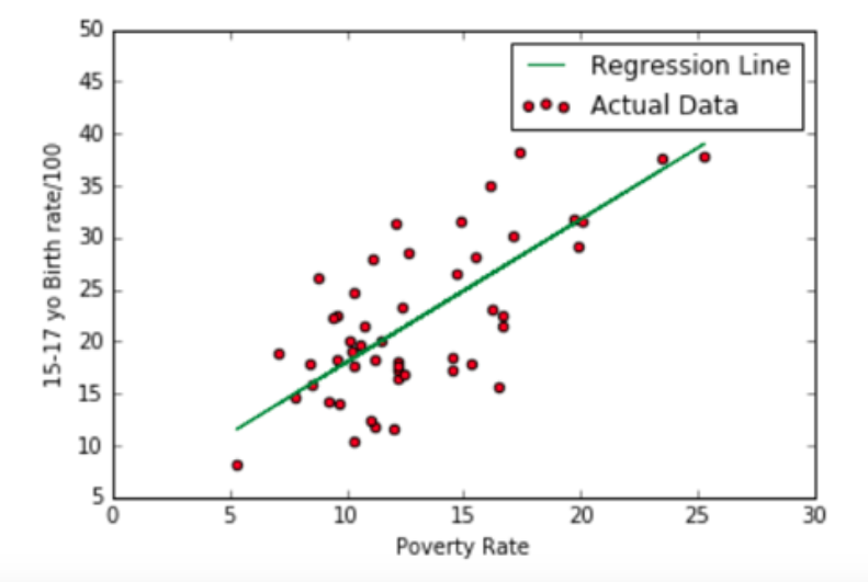
The way to distinguish between classification and regression tasks is to ask whether there is some kind of continuity in the output.
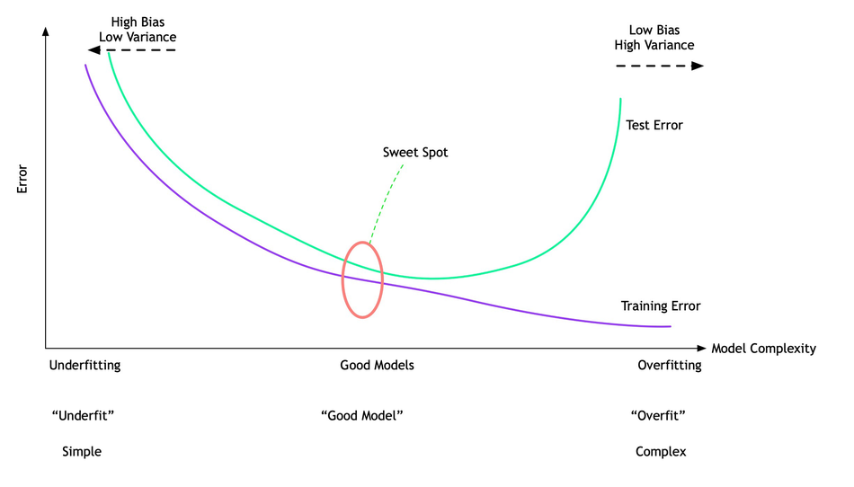
2. Generalization, Overfitting, and Underfitting
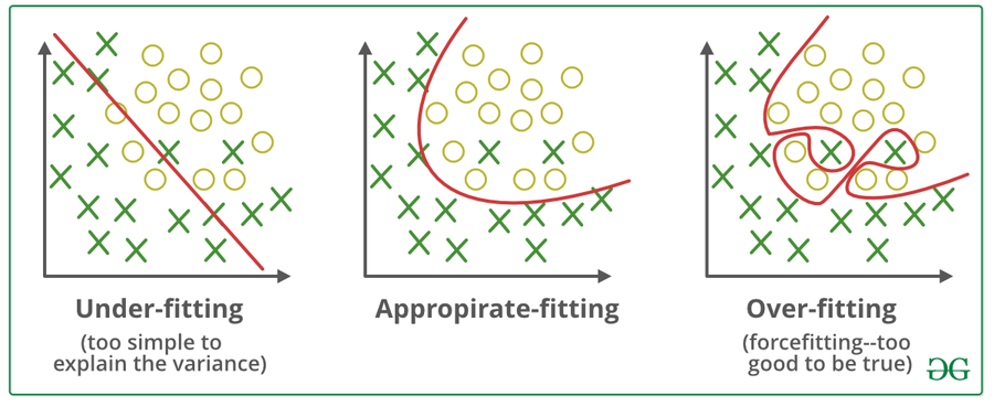
Generalization - Appropriate fitting
- If a model is able to make accurate predictions on unseen data, we say it is able to generalize from the training set to the test set.
Overfiting
- Overfitting occurs when a model too closely to the particularities of the training set and obtain a model that works well on the training set but is not able to generalize to new data.
Underfiting
- Overfitting occurs when model will do badly even on the training set
The complexity of the model: Extensive (cover) capabilities of the model
The more complex we allow our model to be, the better we will be able to predict on the training data.
However, if our model becomes too complex, we start focusing too much on each individual data point in our training set, and the model will not generalize well to new data.
Sweet spot
A point between that will yield the best generalization performance. This is the model we want to find.
3. Relation of Model Complexity to Dataset Size
- The larger variety of data points your dataset contains, the more complex a model you can use without overfitting => data can cover more possible casesthen the model will be more complexity and helpful.
- Larger datasets allow building more complex models.
Note:
- Duplicating the same data points or collecting very similar data will not help.
import mglearn
import matplotlib.pyplot as plt
%matplotlib inline
# generate dataset
X, y = mglearn.datasets.make_forge()
# plot dataset
mglearn.discrete_scatter(X[:, 0], X[:, 1], y)
plt.legend(["Class 0", "Class 1"], loc=4)
plt.xlabel("First feature")
plt.ylabel("Second feature")
print("X.shape:", X.shape)
X, y = mglearn.datasets.make_wave(n_samples=40)
plt.plot(X, y, 'o')
plt.ylim(-3, 3)
plt.xlabel("Feature")
plt.ylabel("Target")
from sklearn.datasets import load_breast_cancer
cancer = load_breast_cancer()
print("cancer.keys():\n", cancer.keys())
print("Shape of cancer data:", cancer.data.shape)
import numpy as np
print("Sample counts per class:\n", {n: v for n, v in zip(cancer.target_names, np.bincount(cancer.target))})
print("Feature names:\n", cancer.feature_names)
from sklearn.datasets import load_boston
boston = load_boston()
print("Data shape:", boston.data.shape)
X, y = mglearn.datasets.load_extended_boston()
print("X.shape:", X.shape)
4.1 k-Nearest Neighbors (KNN)
- KNN make a prediction for a new data point by finding the closest data points in the training dataset
- KNN build the model consists only of storing the training dataset.
4.1.1 k-Neighbors classification
- Consider an arbitrary number, k, of neighbors and assign the class that is more frequent: in other words, the majority class among the k-nearest neighbors
mglearn.plots.plot_knn_classification(n_neighbors=1)
In its simplest version, the k-NN algorithm only considers exactly one nearest neighbor, which is the closest training data point to the point we want to make a prediction for
mglearn.plots.plot_knn_classification(n_neighbors=3)
Instead of considering only the closest neighbor, we can also consider an arbitrary number, k, of neighbors. We use voting to assign a label. This means that for each test point, we count how many neighbors belong to class 0 and how many neighbors belong to class 1. Then assign the class that is more frequent: in other words, the majority class among the k-nearest neighbors
from sklearn.model_selection import train_test_split
X, y = mglearn.datasets.make_forge()

X_train, X_test, y_train, y_test = train_test_split(X, y, random_state=0)
from sklearn.neighbors import KNeighborsClassifier
clf = KNeighborsClassifier(n_neighbors=3)
clf.fit(X_train, y_train)
print("Test set predictions:", clf.predict(X_test))
print("Test set accuracy: {:.2f}".format(clf.score(X_test, y_test)))
Analyzing KNeighborsClassifier
To analyze K-neighbord classifier, we color the plane according to the class that would be assigned to a point in this region, called decision boundary.
fig, axes = plt.subplots(1, 3, figsize=(10, 3))

for n_neighbors, ax in zip([1, 3, 9], axes):
    # the fit method returns the object self, so we can instantiate
    # and fit in one line
    clf = KNeighborsClassifier(n_neighbors=n_neighbors).fit(X, y)
    mglearn.plots.plot_2d_separator(clf, X, fill=True, eps=0.5, ax=ax, alpha=.4)
    mglearn.discrete_scatter(X[:, 0], X[:, 1], y, ax=ax)
    ax.set_title("{} neighbor(s)".format(n_neighbors))
    ax.set_xlabel("feature 0")
    ax.set_ylabel("feature 1")
axes[0].legend(loc=3)
- The decision boundary, which is the divide between where the algorithm assigns class 0 versus where it assigns class 1.
How much k is better?
- We try to tunning k-values to find the best fit for our model.
- We run the KNN algorithm several times with different values of K and choose the K that reduces the number of errors we encounter while maintaining the algorithm’s ability to accurately make predictions when it’s given data it hasn’t seen before.
Note:
As we decrease the value of K to 1, our predictions become less stable. Because K=1, KNN may be incorrectly predicts.
Inversely, as we increase the value of K, our predictions become more stable due to majority voting / averaging, and thus, more likely to make more accurate predictions (up to a certain point).
In cases where we are taking a majority vote among labels, we usually make K an odd number to have a tiebreaker.
from sklearn.datasets import load_breast_cancer

cancer = load_breast_cancer()
X_train, X_test, y_train, y_test = train_test_split(
    cancer.data, cancer.target, stratify=cancer.target, random_state=66)

training_accuracy = []
test_accuracy = []
# try n_neighbors from 1 to 10
neighbors_settings = range(1, 11)

for n_neighbors in neighbors_settings:
    # build the model
    clf = KNeighborsClassifier(n_neighbors=n_neighbors)
    clf.fit(X_train, y_train)
    # record training set accuracy
    training_accuracy.append(clf.score(X_train, y_train))
    # record generalization accuracy
    test_accuracy.append(clf.score(X_test, y_test))

plt.plot(neighbors_settings, training_accuracy, label="training accuracy")
plt.plot(neighbors_settings, test_accuracy, label="test accuracy")
plt.ylabel("Accuracy")
plt.xlabel("n_neighbors")
plt.legend()
- A single neighbor results in a decision boundary that follows the training data closely
- Considering more and more neighbors leads to a smoother decision boundary. A smoother boundary corresponds to a simpler model.
4.1.2 k-neighbors regression
Predictions made by nearest-neighbor regression on the wave dataset
- A simple implementation of KNN regression is to calculate the average of the numerical target of the K nearest neighbors.
- Another approach uses an inverse distance weighted average of the K nearest neighbors.
- KNN regression uses the same distance functions as KNN classification.
mglearn.plots.plot_knn_regression(n_neighbors=1)
mglearn.plots.plot_knn_regression(n_neighbors=3)
from sklearn.neighbors import KNeighborsRegressor

X, y = mglearn.datasets.make_wave(n_samples=40)

# split the wave dataset into a training and a test set
X_train, X_test, y_train, y_test = train_test_split(X, y, random_state=0)

# instantiate the model and set the number of neighbors to consider to 3
reg = KNeighborsRegressor(n_neighbors=3)
# fit the model using the training data and training targets
reg.fit(X_train, y_train)
print("Test set predictions:\n", reg.predict(X_test))
print("Test set R^2: {:.2f}".format(reg.score(X_test, y_test)))
Analyzing KNeighborsRegressor
fig, axes = plt.subplots(1, 3, figsize=(15, 4))
# create 1,000 data points, evenly spaced between -3 and 3
line = np.linspace(-3, 3, 1000).reshape(-1, 1)
for n_neighbors, ax in zip([1, 3, 9], axes):
    # make predictions using 1, 3, or 9 neighbors
    reg = KNeighborsRegressor(n_neighbors=n_neighbors)
    reg.fit(X_train, y_train)
    ax.plot(line, reg.predict(line))
    ax.plot(X_train, y_train, '^', c=mglearn.cm2(0), markersize=8)
    ax.plot(X_test, y_test, 'v', c=mglearn.cm2(1), markersize=8)

    ax.set_title(
        "{} neighbor(s)\n train score: {:.2f} test score: {:.2f}".format(
            n_neighbors, reg.score(X_train, y_train),
            reg.score(X_test, y_test)))
    ax.set_xlabel("Feature")
    ax.set_ylabel("Target")
axes[0].legend(["Model predictions", "Training data/target",
                "Test data/target"], loc="best")
Strengths, weaknesses, and parameters
Strengths:
- The model is very easy to understand,
- Gives reasonable performance without a lot of adjustments.
The nearest neighbors model is usually very fast => good baseline method to try before considering more advanced techniques
Weaknesses:
- Training set is very large (either in number of features or in number of samples) prediction can be slow
- It's Not perform well on datasets with many features
- It does particularly badly with datasets where most features are 0 most of the time(sparse datasets)
Parameters:
- Two important parameters to the KNeighbors classifier:
- The number of neighbors
- Measure distance methods (between data points-Euclidean)
4.2 Linear Models
Linear models make a prediction using a linear function of the input features
Two main types of linear models:
- Regression
- Classification
4.2.1 Linear regression (or ordinary least squares)
- Linear regression will find a straight line that will try to best fit the data provided
X: the features
W: the slope
b: the y-axis offset
mglearn.plots.plot_linear_regression_wave()
Application of linear regression
Linear regression refers to a model that can show relationship between two variables(“dependent variable” and “independent variables”) and how the variation in the “dependent variable” can be captured by change in the “independent variables”.
Independent variables: explain the factors that influence the dependent variable along with the degree of the impact which can be calculated using “parameter estimates” or “coefficients”.
- Linear Regression is a very powerful statistical technique and can be used to generate insights on consumer behaviour, understanding business and factors influencing profitability.
- Linear regression can also be used to analyze the marketing effectiveness, pricing and promotions on sales of a product.
- Linear Regression can be also used to assess risk in financial services or insurance domain.
from sklearn.linear_model import LinearRegression
X, y = mglearn.datasets.make_wave(n_samples=60)
X_train, X_test, y_train, y_test = train_test_split(X, y, random_state=42)

lr = LinearRegression().fit(X_train, y_train)
Random_state ?
- The “slope” parameters (w), also called weights or coefficients, are stored in the coef_attribute
- The offset or intercept (b) is stored in the intercept_ attribute
print("lr.coef_:", lr.coef_)
print("lr.intercept_:", lr.intercept_)
print("Training set score: {:.2f}".format(lr.score(X_train, y_train)))
print("Test set score: {:.2f}".format(lr.score(X_test, y_test)))
X, y = mglearn.datasets.load_extended_boston()

X_train, X_test, y_train, y_test = train_test_split(X, y, random_state=0)
lr = LinearRegression().fit(X_train, y_train)
print("Training set score: {:.2f}".format(lr.score(X_train, y_train)))
print("Test set score: {:.2f}".format(lr.score(X_test, y_test)))
The performance on the training set and the test set is a clear sign of overfitting, and therefore we should try to find a model that allows us to control complexity.
Ridge regression - self reading
- Ridge regression is also a linear model for regression
- The coefficients (w) are chosen not only so that they predict well on the training data, but also to fit an additional constraint.
- Each feature should have as little effect on the outcome as possible (which translates to having a small slope), while still predicting well => Regularization, means explicitly restricting a model to avoid overfitting
from sklearn.linear_model import Ridge

ridge = Ridge().fit(X_train, y_train)
print("Training set score: {:.2f}".format(ridge.score(X_train, y_train)))
print("Test set score: {:.2f}".format(ridge.score(X_test, y_test)))
The Ridge model makes a trade-off between the simplicity of the model (near-zero coefficients) and its performance on the training set. Using the alpha parameter to define the importance of the model places on simplicity and training set performance
ridge10 = Ridge(alpha=10).fit(X_train, y_train)
print("Training set score: {:.2f}".format(ridge10.score(X_train, y_train)))
print("Test set score: {:.2f}".format(ridge10.score(X_test, y_test)))
ridge01 = Ridge(alpha=0.1).fit(X_train, y_train)
print("Training set score: {:.2f}".format(ridge01.score(X_train, y_train)))
print("Test set score: {:.2f}".format(ridge01.score(X_test, y_test)))
Note: We could try decreasing alpha even more to improve generalization.
plt.plot(ridge.coef_, 's', label="Ridge alpha=1")
plt.plot(ridge10.coef_, '^', label="Ridge alpha=10")
plt.plot(ridge01.coef_, 'v', label="Ridge alpha=0.1")

plt.plot(lr.coef_, 'o', label="LinearRegression")
plt.xlabel("Coefficient index")
plt.ylabel("Coefficient magnitude")
xlims = plt.xlim()
plt.hlines(0, xlims[0], xlims[1])
plt.xlim(xlims)
plt.ylim(-25, 25)
plt.legend()
mglearn.plots.plot_ridge_n_samples()
Lasso - self reading
from sklearn.linear_model import Lasso

lasso = Lasso().fit(X_train, y_train)
print("Training set score: {:.2f}".format(lasso.score(X_train, y_train)))
print("Test set score: {:.2f}".format(lasso.score(X_test, y_test)))
print("Number of features used:", np.sum(lasso.coef_ != 0))
# we increase the default setting of "max_iter",
# otherwise the model would warn us that we should increase max_iter.
lasso001 = Lasso(alpha=0.01, max_iter=100000).fit(X_train, y_train)
print("Training set score: {:.2f}".format(lasso001.score(X_train, y_train)))
print("Test set score: {:.2f}".format(lasso001.score(X_test, y_test)))
print("Number of features used:", np.sum(lasso001.coef_ != 0))
lasso00001 = Lasso(alpha=0.0001, max_iter=100000).fit(X_train, y_train)
print("Training set score: {:.2f}".format(lasso00001.score(X_train, y_train)))
print("Test set score: {:.2f}".format(lasso00001.score(X_test, y_test)))
print("Number of features used:", np.sum(lasso00001.coef_ != 0))
plt.plot(lasso.coef_, 's', label="Lasso alpha=1")
plt.plot(lasso001.coef_, '^', label="Lasso alpha=0.01")
plt.plot(lasso00001.coef_, 'v', label="Lasso alpha=0.0001")

plt.plot(ridge01.coef_, 'o', label="Ridge alpha=0.1")
plt.legend(ncol=2, loc=(0, 1.05))
plt.ylim(-25, 25)
plt.xlabel("Coefficient index")
plt.ylabel("Coefficient magnitude")
4.2.2 Linear models for classification
The formula looks very similar to the one for linear regression, but instead we threshold the predicted value at zero.
- The function is smaller than zero, we predict the class –1;
- The function is larger than zero, we predict the class +1.
The two most common linear classification algorithms:
- Logistic regression
- Linear support vector machines (linear SVMs) \begin{align*} \end{align*}
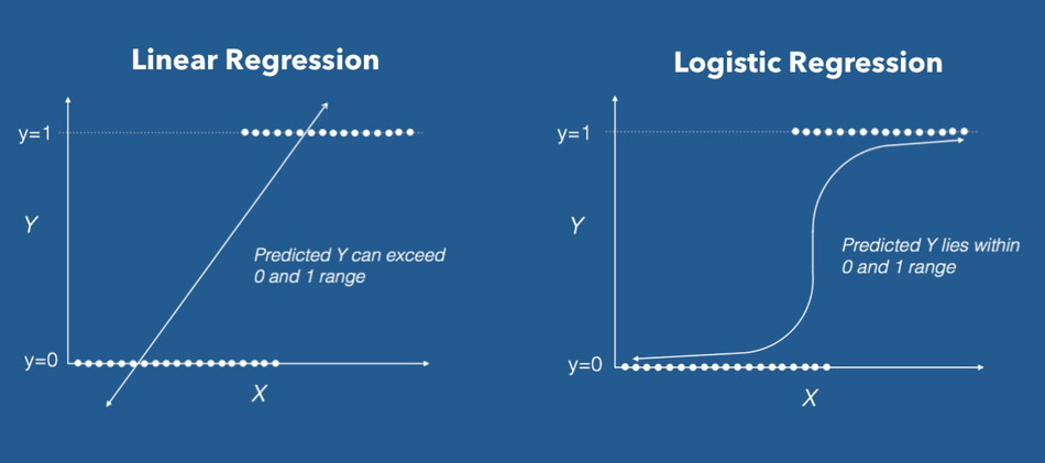
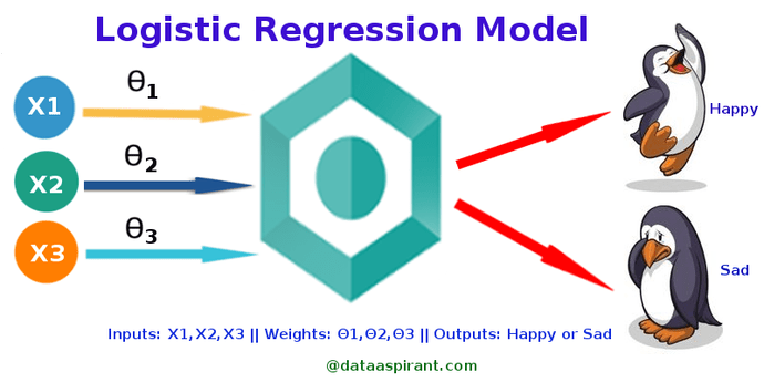
4.2.2.1 Logistic regression
- Logistic Regression is a Machine Learning algorithm which is used for the classification problems, it is a predictive analysis algorithm and based on the concept of probability.
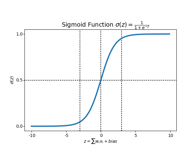
Sigmoid function
- Regression uses ‘Sigmoid function’ or also known as the ‘logistic function’. Sigmoid function maps any real value into another value between 0 and 1, we use sigmoid to map predictions to probabilities.
Logistic regression applications:
- Spam Detection
- The Credit Card Fraud Detection problem
- Tumour Prediction
- Marketing: customer like a new product ? .........
4.2.2.2 Linear support vector machines
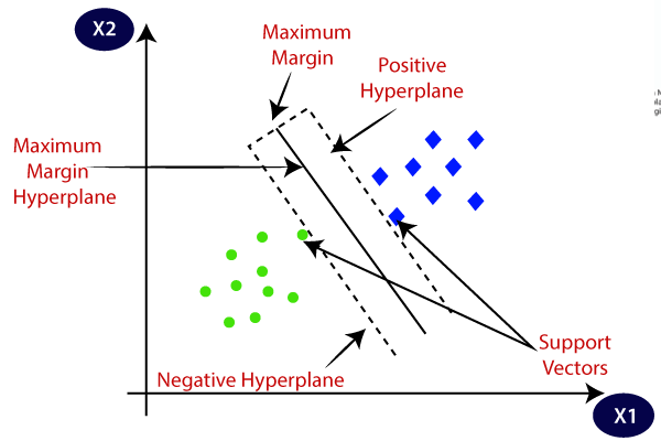
The objective of the support vector machine algorithm is to find a hyperplane in an N-dimensional space(N — the number of features) that distinctly classifies the data points.
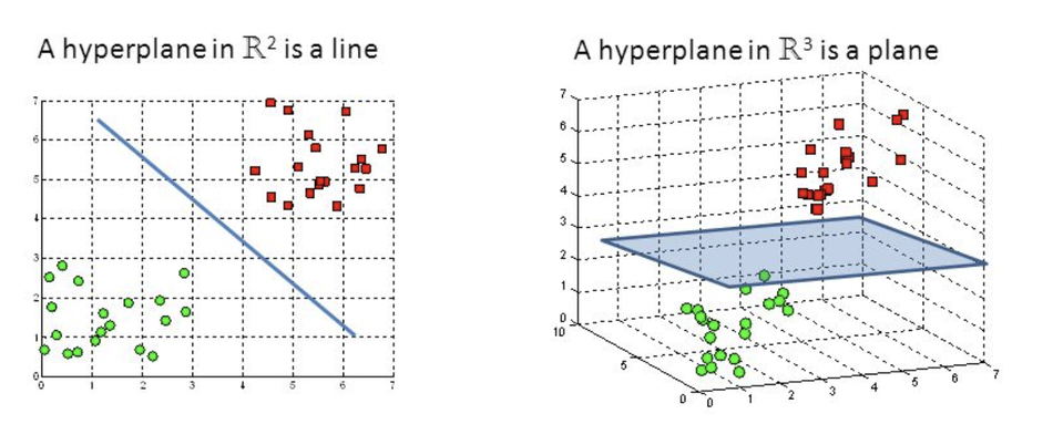
Hyperplanes
Hyperplanes are decision boundaries that help classify the data points. Data points falling on either side of the hyperplane can be attributed to different classes.
Support vector
Support vectors are data points that are closer to the hyperplane and influence the position and orientation of the hyperplane.
from sklearn.linear_model import LogisticRegression
from sklearn.svm import LinearSVC

X, y = mglearn.datasets.make_forge()

fig, axes = plt.subplots(1, 2, figsize=(10, 3))

for model, ax in zip([LinearSVC(), LogisticRegression()], axes):
    clf = model.fit(X, y)
    mglearn.plots.plot_2d_separator(clf, X, fill=False, eps=0.5,
                                    ax=ax, alpha=.7)
    mglearn.discrete_scatter(X[:, 0], X[:, 1], y, ax=ax)
    ax.set_title(clf.__class__.__name__)
    ax.set_xlabel("Feature 0")
    ax.set_ylabel("Feature 1")
axes[0].legend()
mglearn.plots.plot_linear_svc_regularization()
from sklearn.datasets import load_breast_cancer
cancer = load_breast_cancer()
X_train, X_test, y_train, y_test = train_test_split(
    cancer.data, cancer.target, stratify=cancer.target, random_state=42)
logreg = LogisticRegression().fit(X_train, y_train)
print("Training set score: {:.3f}".format(logreg.score(X_train, y_train)))
print("Test set score: {:.3f}".format(logreg.score(X_test, y_test)))
logreg100 = LogisticRegression(C=100).fit(X_train, y_train)
print("Training set score: {:.3f}".format(logreg100.score(X_train, y_train)))
print("Test set score: {:.3f}".format(logreg100.score(X_test, y_test)))
logreg001 = LogisticRegression(C=0.01).fit(X_train, y_train)
print("Training set score: {:.3f}".format(logreg001.score(X_train, y_train)))
print("Test set score: {:.3f}".format(logreg001.score(X_test, y_test)))
For LogisticRegression and LinearSVC the trade-off parameter that determines the strength of the regularization is called C, and higher values of C correspond to less regularization.
- A high value for the parameter C, we try to fit the training set as best as possible,
- A low values of the parameter C, the models put more emphasis on finding a coefficient vector (w) that is close to zero.
plt.plot(logreg.coef_.T, 'o', label="C=1")
plt.plot(logreg100.coef_.T, '^', label="C=100")
plt.plot(logreg001.coef_.T, 'v', label="C=0.001")
plt.xticks(range(cancer.data.shape[1]), cancer.feature_names, rotation=90)
xlims = plt.xlim()
plt.hlines(0, xlims[0], xlims[1])
plt.xlim(xlims)
plt.ylim(-5, 5)
plt.xlabel("Feature")
plt.ylabel("Coefficient magnitude")
plt.legend()
for C, marker in zip([0.001, 1, 100], ['o', '^', 'v']):
    lr_l1 = LogisticRegression(C=C, solver='liblinear', penalty="l1").fit(X_train, y_train)
    print("Training accuracy of l1 logreg with C={:.3f}: {:.2f}".format(
          C, lr_l1.score(X_train, y_train)))
    print("Test accuracy of l1 logreg with C={:.3f}: {:.2f}".format(
          C, lr_l1.score(X_test, y_test)))
    plt.plot(lr_l1.coef_.T, marker, label="C={:.3f}".format(C))

plt.xticks(range(cancer.data.shape[1]), cancer.feature_names, rotation=90)
xlims = plt.xlim()
plt.hlines(0, xlims[0], xlims[1])
plt.xlim(xlims)
plt.xlabel("Feature")
plt.ylabel("Coefficient magnitude")

plt.ylim(-5, 5)
plt.legend(loc=3)
Linear models for multiclass classification
- All binary classifiers are run on a test point
- The classifier that has the highest score on its single class “wins,” and this class label is returned as the prediction. \begin{align*} \end{align*}
from sklearn.datasets import make_blobs

X, y = make_blobs(random_state=42)
mglearn.discrete_scatter(X[:, 0], X[:, 1], y)
plt.xlabel("Feature 0")
plt.ylabel("Feature 1")
plt.legend(["Class 0", "Class 1", "Class 2"])
linear_svm = LinearSVC().fit(X, y)
print("Coefficient shape: ", linear_svm.coef_.shape)
print("Intercept shape: ", linear_svm.intercept_.shape)
mglearn.discrete_scatter(X[:, 0], X[:, 1], y)
line = np.linspace(-15, 15)
for coef, intercept, color in zip(linear_svm.coef_, linear_svm.intercept_,
                                  mglearn.cm3.colors):
    plt.plot(line, -(line * coef[0] + intercept) / coef[1], c=color)
plt.ylim(-10, 15)
plt.xlim(-10, 8)
plt.xlabel("Feature 0")
plt.ylabel("Feature 1")
plt.legend(['Class 0', 'Class 1', 'Class 2', 'Line class 0', 'Line class 1',
            'Line class 2'], loc=(1.01, 0.3))
mglearn.plots.plot_2d_classification(linear_svm, X, fill=True, alpha=.7)
mglearn.discrete_scatter(X[:, 0], X[:, 1], y)
line = np.linspace(-15, 15)
for coef, intercept, color in zip(linear_svm.coef_, linear_svm.intercept_,
                                  mglearn.cm3.colors):
    plt.plot(line, -(line * coef[0] + intercept) / coef[1], c=color)
plt.legend(['Class 0', 'Class 1', 'Class 2', 'Line class 0', 'Line class 1',
            'Line class 2'], loc=(1.01, 0.3))
plt.xlabel("Feature 0")
plt.ylabel("Feature 1")
We accomplish this by using the softmax function. ???
Strengths, weaknesses and parameters
Parameters:
- The main parameter of linear models is the regularization parameter, called alpha in the regression models and C in LinearSVC and LogisticRegression. Large values for alpha or small values for C mean simple models.
- The other decision you have to make is whether you want to use L1 regularization or L2 regularization. If you assume that only a few of your features are actually important, you should use L1. Otherwise, you should default to L2
Strengths:
- Very fast to train, and also fast to predict.
- Easy to understand how a prediction is made => Explain the relationship between dependence and independence variables.
- Used in large datasets.
Weaknesses:
- Dataset has highly correlated features => the coefficients might be hard to interpret
- Not good in lower-dimensional spaces
# instantiate model and fit it in one line
logreg = LogisticRegression().fit(X_train, y_train)
logreg = LogisticRegression()
y_pred = logreg.fit(X_train, y_train).predict(X_test)
y_pred = LogisticRegression().fit(X_train, y_train).predict(X_test)
4.3 Naive Bayes Classifiers
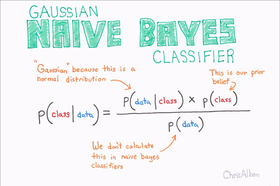
Naive Bayes classifiers are a collection of classification algorithms based on Bayes’ Theorem. It is not a single algorithm but a family of algorithms where all of them share a common principle, i.e. every pair of features being classified is independent of each other.
Naive Bayes is a classification algorithm for binary (two-class) and multi-class classification problems.
The technique is easiest to understand when described using binary or categorical input values.
X = np.array([[0, 1, 0, 1],
              [1, 0, 1, 1],
              [0, 0, 0, 1],
              [1, 0, 1, 0]])
y = np.array([0, 1, 0, 1])
- To make a prediction, a data point is compared to the statistics for each of the classes, and the best matching class is predicted.
counts = {}
for label in np.unique(y):
    # iterate over each class
    # count (sum) entries of 1 per feature
    counts[label] = X[y == label].sum(axis=0)
print("Feature counts:\n", counts)
Note: The reason that naive Bayes models are so efficient is that they learn parameters by looking at each feature individually and collect simple per-class statistics from each feature
Strengths, weaknesses and parameters
Strengths:
- Very fast to train and to predict, and the training procedure is easy to understand.
- The models work very well with high-dimensional sparse data and are relatively robust to the parameters.
- Naive Bayes models are great baseline models and are often used on very large datasets
Weaknesses:
- If categorical variable has a category (in test data set), which was not observed in training data set, then model will assign a 0 (zero) probability and will be unable to make a prediction.
4.4 Decision trees
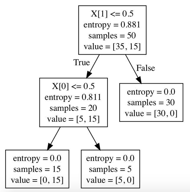
- In decision analysis, a decision tree can be used to visually and explicitly represent decisions and decision making.
- A decision tree is a tree where each node represents a feature(attribute), each link(branch) represents a decision(rule) and each leaf represents an outcome(categorical or continues value)
# mglearn.plots.plot_animal_tree()
The reasons have to choose Decision tree
Decision tress often mimic the human level thinking so its so simple to understand the data and make some good interpretations.
Decision trees actually make you see the logic for the data to interpret
How to make Decision tree
Entropy: is the measure of the amount of uncertainty or randomness in data.
- High entropy => low predictability
- Low entropy => high predictability
Information Gain: is the effective change in entropy after deciding on a particular attribute A. It measures the relative change in entropy with respect to the independent variables.
Building decision trees
mglearn.plots.plot_tree_progressive()
How to make Decision tree: Step by steps
- Create root node for the tree
- If all examples are positive, return leaf node ‘positive’
- Else if all examples are negative, return leaf node ‘negative’
- Calculate the entropy of current state H(S)
- For each attribute, calculate the entropy with respect to the attribute ‘x’ denoted by H(S, x)
- Select the attribute which has maximum value of IG(S, x)
- Remove the attribute that offers highest IG from the set of attributes
- Repeat until we run out of all attributes, or the decision tree has all leaf nodes.
Controlling complexity of decision trees
from sklearn.tree import DecisionTreeClassifier
from sklearn.datasets import load_breast_cancer
from sklearn.model_selection import train_test_split

cancer = load_breast_cancer()
X_train, X_test, y_train, y_test = train_test_split(
    cancer.data, cancer.target, stratify=cancer.target, random_state=42)
tree_ = DecisionTreeClassifier(random_state=0)
tree_.fit(X_train, y_train)
print("Accuracy on training set: {:.3f}".format(tree.score(X_train, y_train)))
print("Accuracy on test set: {:.3f}".format(tree.score(X_test, y_test)))
tree_ = DecisionTreeClassifier(max_depth=4, random_state=0)
tree_.fit(X_train, y_train)

print("Accuracy on training set: {:.3f}".format(tree_.score(X_train, y_train)))
print("Accuracy on test set: {:.3f}".format(tree_.score(X_test, y_test)))
There are two common strategies to prevent overfitting:
- Stopping the creation of the tree early (also called pre-pruning), include limiting the maximum depth of the tree, limiting the maximum number of leaves, or requiring a minimum number of points in a node to keep splitting it.
- Building the tree but then removing or collapsing nodes that contain little information (also called post-pruning or just pruning).
Analyzing Decision Trees
The visualization of the tree provides a great in-depth view of how the algorithm makes predictions, and is a good example of a machine learning algorithm that is easily explained to nonexperts
from sklearn.tree import export_graphviz
dot_data = export_graphviz(tree_, out_file="tree.dot", class_names=["malignant", "benign"],
                feature_names=cancer.feature_names, impurity=False, filled=True)
import graphviz

with open('tree.dot') as f:
    dot_graph = f.read()
graphviz.Source(dot_graph)
Feature Importance in trees
- The most commonly used summary is feature importance, which rates how important each feature is for the decision a tree makes.
- It is a number between 0 and 1 for each feature, where 0 means “not used at all” and 1 means perfectly predicts the target.” The feature importances always sum to 1
print("Feature importances:")
print(tree.feature_importances_)
def plot_feature_importances_cancer(model):
    n_features = cancer.data.shape[1]
    plt.barh(np.arange(n_features), model.feature_importances_, align='center')
    plt.yticks(np.arange(n_features), cancer.feature_names)
    plt.xlabel("Feature importance")
    plt.ylabel("Feature")
    plt.ylim(-1, n_features)

plot_feature_importances_cancer(tree)
tree = mglearn.plots.plot_tree_not_monotone()
display(tree)
import os
ram_prices = pd.read_csv(os.path.join(mglearn.datasets.DATA_PATH, "ram_price.csv"))

plt.semilogy(ram_prices.date, ram_prices.price)
plt.xlabel("Year")
plt.ylabel("Price in $/Mbyte")
from sklearn.tree import DecisionTreeRegressor
# use historical data to forecast prices after the year 2000
data_train = ram_prices[ram_prices.date < 2000]
data_test = ram_prices[ram_prices.date >= 2000]

# predict prices based on date
X_train = data_train.date[:, np.newaxis]
# we use a log-transform to get a simpler relationship of data to target
y_train = np.log(data_train.price)

tree = DecisionTreeRegressor(max_depth=3).fit(X_train, y_train)
linear_reg = LinearRegression().fit(X_train, y_train)

# predict on all data
X_all = ram_prices.date[:, np.newaxis]

pred_tree = tree.predict(X_all)
pred_lr = linear_reg.predict(X_all)

# undo log-transform
price_tree = np.exp(pred_tree)
price_lr = np.exp(pred_lr)
plt.semilogy(data_train.date, data_train.price, label="Training data")
plt.semilogy(data_test.date, data_test.price, label="Test data")
plt.semilogy(ram_prices.date, price_tree, label="Tree prediction")
plt.semilogy(ram_prices.date, price_lr, label="Linear prediction")
plt.legend()
Strengths, weaknesses and parameters
Strengths:
- The resulting model can easily be visualized and understood by nonexperts (at least for smaller trees),
- The algorithms are completely invariant to scaling of the data.
Weaknesses:
- The main downside of decision trees is that even with the use of pre-pruning, they tend to overfit and provide poor generalization performance
Parameters:
- the parameters that control model complexity in decision trees are the pre-pruning parameters that stop the building of the tree before it is fully developed. max_depth, max_leaf_nodes, or min_samples_leaf—is sufficient to prevent overfitting.
Ensembles of Decision Trees
Ensembles are methods that combine multiple machine learning models to create more powerful models.
- Two ensemble models that have proven to be effective on a wide range of datasets for classification and regressiondecision trees:
- Random forests
- Gradient boosted decision trees.
4.5 Random forests
Random forests are one way to address overfitting problem of decission tree.
A random forest is essentially a collection of decision trees, where each tree is slightly different from the others.
- Build many trees, all of which work well and overfit in different ways, we can reduce the amount of overfitting by averaging their results
Building random forests
Step by step:
- Decide on the number of trees to build: These trees will be built completely independently from each other
- For a tree, we first take bootstrap sample of our data. From n_samples, take an example randomly with replacement n_time => create a new dataset = the original dataset.
- A decision tree is built based on this newly created dataset.
- Repeat step 2 until enough decided tree
The probabilities predicted by all the trees are averaged, and the class with the highest probability is predicted.
Analyzing random forests
from sklearn.ensemble import RandomForestClassifier
from sklearn.datasets import make_moons

X, y = make_moons(n_samples=100, noise=0.25, random_state=3)
X_train, X_test, y_train, y_test = train_test_split(X, y, stratify=y,
                                                    random_state=42)

forest = RandomForestClassifier(n_estimators=5, random_state=2)
forest.fit(X_train, y_train)
fig, axes = plt.subplots(2, 3, figsize=(20, 10))
for i, (ax, tree) in enumerate(zip(axes.ravel(), forest.estimators_)):
    ax.set_title("Tree {}".format(i))
    mglearn.plots.plot_tree_partition(X_train, y_train, tree, ax=ax)

mglearn.plots.plot_2d_separator(forest, X_train, fill=True, ax=axes[-1, -1],
                                alpha=.4)
axes[-1, -1].set_title("Random Forest")
mglearn.discrete_scatter(X_train[:, 0], X_train[:, 1], y_train)
X_train, X_test, y_train, y_test = train_test_split(
    cancer.data, cancer.target, random_state=0)
forest = RandomForestClassifier(n_estimators=100, random_state=0)
forest.fit(X_train, y_train)

print("Accuracy on training set: {:.3f}".format(forest.score(X_train, y_train)))
print("Accuracy on test set: {:.3f}".format(forest.score(X_test, y_test)))
plot_feature_importances_cancer(forest)
- The random forest gives nonzero importance to many more features than the single tree.
- The random forest consider many possible explanations, the result being that the random forest captures a much broader picture of the data than a single tree.
Strengths, weaknesses, and parameters
4.6 Gradient Boosted Regression Trees (Gradient Boosting Machines)
- Gradient boosting works by building trees in a serial manner, where each tree tries to correct the mistakes of the previous one
- Used for regression and classification
- Provide better accuracy if the parameters are set correctly.
- The pre-pruning: limiting the maximum depth (max_depth)
- The number of trees in the ensemble (the same with random forest)
- The learning_rate: controls how strongly each tree tries to correct the mistakes of the previous trees
- A higher learning rate means each tree can make stronger corrections, allowing for more complex models.
- A lower the learning rate only increased the generalization performance slightly
from sklearn.ensemble import GradientBoostingClassifier

X_train, X_test, y_train, y_test = train_test_split(
    cancer.data, cancer.target, random_state=0)

gbrt = GradientBoostingClassifier(random_state=0)
gbrt.fit(X_train, y_train)

print("Accuracy on training set: {:.3f}".format(gbrt.score(X_train, y_train)))
print("Accuracy on test set: {:.3f}".format(gbrt.score(X_test, y_test)))
gbrt = GradientBoostingClassifier(random_state=0, max_depth=1)
gbrt.fit(X_train, y_train)

print("Accuracy on training set: {:.3f}".format(gbrt.score(X_train, y_train)))
print("Accuracy on test set: {:.3f}".format(gbrt.score(X_test, y_test)))
gbrt = GradientBoostingClassifier(random_state=0, learning_rate=0.01)
gbrt.fit(X_train, y_train)

print("Accuracy on training set: {:.3f}".format(gbrt.score(X_train, y_train)))
print("Accuracy on test set: {:.3f}".format(gbrt.score(X_test, y_test)))
gbrt = GradientBoostingClassifier(random_state=0, max_depth=1)
gbrt.fit(X_train, y_train)

plot_feature_importances_cancer(gbrt)
Strengths, weaknesses and parameters
4.7 Kernelized Support Vector Machines
- Kernelized support vector machines (often just referred to as SVMs) are an extension that allows for more complex models that are not defined simply by hyperplanes in the input space.
Linear Models and Non-linear Features
- Linear models can be quite limiting in low-dimensional spaces, as lines and hyperplanes have limited flexibility => need adding more features
X, y = make_blobs(centers=4, random_state=8)
y = y % 2

mglearn.discrete_scatter(X[:, 0], X[:, 1], y)
plt.xlabel("Feature 0")
plt.ylabel("Feature 1")
A linear model for classification can only separate points using a line, and will not be able to do a very good job on above dataset
from sklearn.svm import LinearSVC
linear_svm = LinearSVC().fit(X, y)

mglearn.plots.plot_2d_separator(linear_svm, X)
mglearn.discrete_scatter(X[:, 0], X[:, 1], y)
plt.xlabel("Feature 0")
plt.ylabel("Feature 1")
# add the squared first feature
X_new = np.hstack([X, X[:, 1:] ** 2])


from mpl_toolkits.mplot3d import Axes3D, axes3d
figure = plt.figure()
# visualize in 3D
ax = Axes3D(figure, elev=-152, azim=-26)
# plot first all the points with y==0, then all with y == 1
mask = y == 0
ax.scatter(X_new[mask, 0], X_new[mask, 1], X_new[mask, 2], c='b',
           cmap=mglearn.cm2, s=60, edgecolor='k')
ax.scatter(X_new[~mask, 0], X_new[~mask, 1], X_new[~mask, 2], c='r', marker='^',
           cmap=mglearn.cm2, s=60, edgecolor='k')
ax.set_xlabel("feature0")
ax.set_ylabel("feature1")
ax.set_zlabel("feature1 ** 2")
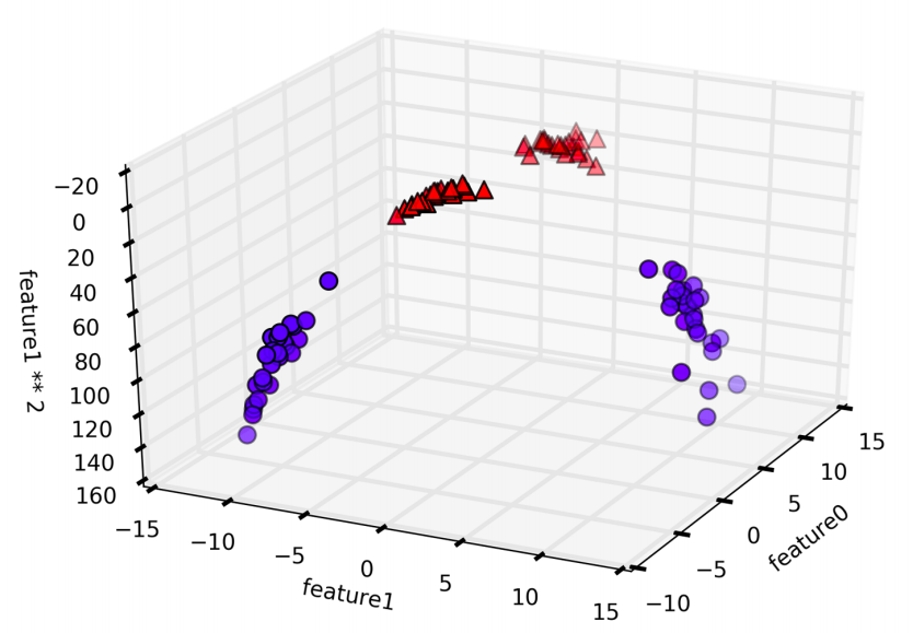
By adding another dimention, now indeed possible to separate the two classes using a linear model, a plane in three dimensions.
linear_svm_3d = LinearSVC().fit(X_new, y)
coef, intercept = linear_svm_3d.coef_.ravel(), linear_svm_3d.intercept_

# show linear decision boundary
figure = plt.figure()
ax = Axes3D(figure, elev=-152, azim=-26)
xx = np.linspace(X_new[:, 0].min() - 2, X_new[:, 0].max() + 2, 50)
yy = np.linspace(X_new[:, 1].min() - 2, X_new[:, 1].max() + 2, 50)

XX, YY = np.meshgrid(xx, yy)
ZZ = (coef[0] * XX + coef[1] * YY + intercept) / -coef[2]
ax.plot_surface(XX, YY, ZZ, rstride=8, cstride=8, alpha=0.3)
ax.scatter(X_new[mask, 0], X_new[mask, 1], X_new[mask, 2], c='b',
           cmap=mglearn.cm2, s=60, edgecolor='k')
ax.scatter(X_new[~mask, 0], X_new[~mask, 1], X_new[~mask, 2], c='r', marker='^',
           cmap=mglearn.cm2, s=60, edgecolor='k')

ax.set_xlabel("feature0")
ax.set_ylabel("feature1")
ax.set_zlabel("feature1 ** 2")
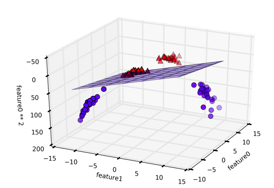
ZZ = YY ** 2
dec = linear_svm_3d.decision_function(np.c_[XX.ravel(), YY.ravel(), ZZ.ravel()])
plt.contourf(XX, YY, dec.reshape(XX.shape), levels=[dec.min(), 0, dec.max()],
             cmap=mglearn.cm2, alpha=0.5)
mglearn.discrete_scatter(X[:, 0], X[:, 1], y)
plt.xlabel("Feature 0")
plt.ylabel("Feature 1")
The Kernel Trick
Adding nonlinear features to the representation of our data can make linear models much more powerful. But we don't know which features to add, adding many features (like all possible interactions in a 100-dimensional feature space) might make computation very expensive.
=> The kernel trick allows us to learn a classifier in a higher-dimensional space without actually computing the new
Two ways to map data into a higher-dimensional space:
- The polynomial kernel, which computes all possible polynomials up to a certain degree of the original features
- The radial basis function (RBF) kernel or Gaussian kernel - put a factor for each feature base on feature' importance as gaussian line
Understanding SVMs
During training, the SVM learns how important each of the training data points is to represent the decision boundary between the two classes.
- SVMs defining the decision boundary: the data point that lie on the border between the classes => support vectors and give the support vector machine its name.
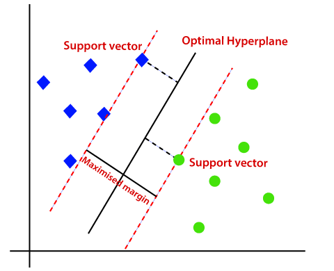
- To make a prediction for a new point, the distance to each of the support vectors is measured.
- A classification decision is made based on the distances to the support vector.
- The importance of the support vectors that was also learned during training.
from sklearn.svm import SVC

X, y = mglearn.tools.make_handcrafted_dataset()
svm = SVC(kernel='rbf', C=10, gamma=0.1).fit(X, y)
mglearn.plots.plot_2d_separator(svm, X, eps=.5)
mglearn.discrete_scatter(X[:, 0], X[:, 1], y)
# plot support vectors
sv = svm.support_vectors_
# class labels of support vectors are given by the sign of the dual coefficients
sv_labels = svm.dual_coef_.ravel() > 0
mglearn.discrete_scatter(sv[:, 0], sv[:, 1], sv_labels, s=15, markeredgewidth=3)
plt.xlabel("Feature 0")
plt.ylabel("Feature 1")
Tuning SVM parameters
- The gamma parameter is controls the width of the Gaussian kernel => determines the scale of what it means for points to be close together
- A small gamma => many points are considered close by
- A low value of gamma => model of low complexity
- A high value of gamma => more complex model.
- The C parameter is a regularization parameter, similar to that used in the linear models.
- A small C means a very restricted model => each data point can only have very limited influence
- Increasing C, allows these points to have a stronger influence on the model and makes the decision boundary bend to correctly classify them.
C and gamma should be adjusted together.
fig, axes = plt.subplots(3, 3, figsize=(15, 10))

for ax, C in zip(axes, [-1, 0, 3]):
    for a, gamma in zip(ax, range(-1, 2)):
        mglearn.plots.plot_svm(log_C=C, log_gamma=gamma, ax=a)

axes[0, 0].legend(["class 0", "class 1", "sv class 0", "sv class 1"],
                  ncol=4, loc=(.9, 1.2))
X_train, X_test, y_train, y_test = train_test_split(
    cancer.data, cancer.target, random_state=0)

svc = SVC()
svc.fit(X_train, y_train)

print("Accuracy on training set: {:.2f}".format(svc.score(X_train, y_train)))
print("Accuracy on test set: {:.2f}".format(svc.score(X_test, y_test)))
plt.boxplot(X_train, manage_xticks=False)
plt.yscale("symlog")
plt.xlabel("Feature index")
plt.ylabel("Feature magnitude")
Preprocessing data for SVMs
# Compute the minimum value per feature on the training set
min_on_training = X_train.min(axis=0)
# Compute the range of each feature (max - min) on the training set
range_on_training = (X_train - min_on_training).max(axis=0)

# subtract the min, divide by range
# afterward, min=0 and max=1 for each feature
X_train_scaled = (X_train - min_on_training) / range_on_training
print("Minimum for each feature\n", X_train_scaled.min(axis=0))
print("Maximum for each feature\n", X_train_scaled.max(axis=0))
# use THE SAME transformation on the test set,
# using min and range of the training set. See Chapter 3 (unsupervised learning) for details.
X_test_scaled = (X_test - min_on_training) / range_on_training
svc = SVC()
svc.fit(X_train_scaled, y_train)

print("Accuracy on training set: {:.3f}".format(
        svc.score(X_train_scaled, y_train)))
print("Accuracy on test set: {:.3f}".format(svc.score(X_test_scaled, y_test)))
svc = SVC(C=1000)
svc.fit(X_train_scaled, y_train)

print("Accuracy on training set: {:.3f}".format(
    svc.score(X_train_scaled, y_train)))
print("Accuracy on test set: {:.3f}".format(svc.score(X_test_scaled, y_test)))
Strengths, weaknesses and parameters
4.8 Neural Networks (Deep Learning)
A family of algorithms known as neural networks model
The Neural Network Model

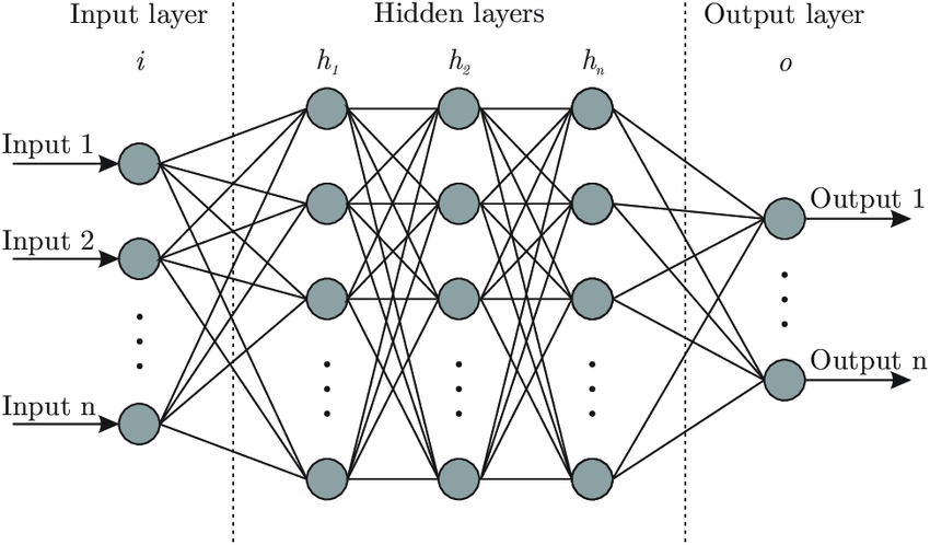
display(mglearn.plots.plot_logistic_regression_graph())
display(mglearn.plots.plot_single_hidden_layer_graph())
line = np.linspace(-3, 3, 100)
plt.plot(line, np.tanh(line), label="tanh")
plt.plot(line, np.maximum(line, 0), label="relu")
plt.legend(loc="best")
plt.xlabel("x")
plt.ylabel("relu(x), tanh(x)")
mglearn.plots.plot_two_hidden_layer_graph()
Tuning Neural Networks
from sklearn.neural_network import MLPClassifier
from sklearn.datasets import make_moons

X, y = make_moons(n_samples=100, noise=0.25, random_state=3)

X_train, X_test, y_train, y_test = train_test_split(X, y, stratify=y,
                                                    random_state=42)
#default the number of hidden nodes is 100
mlp = MLPClassifier(solver='lbfgs', random_state=0).fit(X_train, y_train)

mglearn.plots.plot_2d_separator(mlp, X_train, fill=True, alpha=.3)
mglearn.discrete_scatter(X_train[:, 0], X_train[:, 1], y_train)
plt.xlabel("Feature 0")
plt.ylabel("Feature 1")
mlp = MLPClassifier(solver='lbfgs', random_state=0, hidden_layer_sizes=[10])
mlp.fit(X_train, y_train)
mglearn.plots.plot_2d_separator(mlp, X_train, fill=True, alpha=.3)
mglearn.discrete_scatter(X_train[:, 0], X_train[:, 1], y_train)
plt.xlabel("Feature 0")
plt.ylabel("Feature 1")
# using two hidden layers, with 10 units each
mlp = MLPClassifier(solver='lbfgs', random_state=0,
                    hidden_layer_sizes=[10, 10])
mlp.fit(X_train, y_train)
mglearn.plots.plot_2d_separator(mlp, X_train, fill=True, alpha=.3)
mglearn.discrete_scatter(X_train[:, 0], X_train[:, 1], y_train)
plt.xlabel("Feature 0")
plt.ylabel("Feature 1")
Activation function:
1. Role of the Activation Function in a Neural Network Model
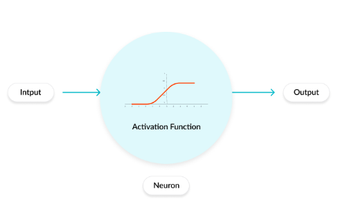
- The activation function is a mathematical “gate” in between the input feeding the current neuron and its output going to the next layer. It can be as simple as a step function that turns the neuron output on and off, depending on a rule or threshold.
- It can be a transformation that maps the input signals into output signals that are needed for the neural network to function.
Most popular types of Activation functions
- Sigmoid or Logistic
- Tanh — Hyperbolic tangent
- ReLu -Rectified linear units

Sigmoid Activation function
- Its Range is between 0 and 1
- It is easy to understand and apply
- But:
- Vanishing gradient problem => saturate and kill gradients.
- It makes the gradient updates go too far in different directions. 0 < output < 1, and it makes optimization harder => slow convergence
Hyperbolic Tangent function- Tanh
- Its range in between -1 to 1 (-1 < output < 1)
- Optimization is easier in this method hence in practice it is always preferred over Sigmoid function.
- But:
- Still it suffers from Vanishing gradient problem.
ReLu- Rectified Linear units
- It’s just R(x) = max(0,x)
- x < 0 , R(x) = 0
- x >= 0 , R(x) = x.
- It is very simple and efficinent.
- Avoids and rectifies vanishing gradient problem
Activation function for output layer:
- Softmax function for a Classification problem to compute the probabilites for the classes.
- Linear function for a regression problem.
# using two hidden layers, with 10 units each, now with tanh nonlinearity.
mlp = MLPClassifier(solver='lbfgs', activation='tanh',
                    random_state=0, hidden_layer_sizes=[10, 10])
mlp.fit(X_train, y_train)
mglearn.plots.plot_2d_separator(mlp, X_train, fill=True, alpha=.3)
mglearn.discrete_scatter(X_train[:, 0], X_train[:, 1], y_train)
plt.xlabel("Feature 0")
plt.ylabel("Feature 1")
fig, axes = plt.subplots(2, 4, figsize=(20, 8))
for axx, n_hidden_nodes in zip(axes, [10, 100]):
    for ax, alpha in zip(axx, [0.0001, 0.01, 0.1, 1]):
        mlp = MLPClassifier(solver='lbfgs', random_state=0,
                            hidden_layer_sizes=[n_hidden_nodes, n_hidden_nodes],
                            alpha=alpha)
        mlp.fit(X_train, y_train)
        mglearn.plots.plot_2d_separator(mlp, X_train, fill=True, alpha=.3, ax=ax)
        mglearn.discrete_scatter(X_train[:, 0], X_train[:, 1], y_train, ax=ax)
        ax.set_title("n_hidden=[{}, {}]\nalpha={:.4f}".format(
                      n_hidden_nodes, n_hidden_nodes, alpha))
fig, axes = plt.subplots(2, 4, figsize=(20, 8))
for i, ax in enumerate(axes.ravel()):
    mlp = MLPClassifier(solver='lbfgs', random_state=i,
                        hidden_layer_sizes=[100, 100])
    mlp.fit(X_train, y_train)
    mglearn.plots.plot_2d_separator(mlp, X_train, fill=True, alpha=.3, ax=ax)
    mglearn.discrete_scatter(X_train[:, 0], X_train[:, 1], y_train, ax=ax)
print("Cancer data per-feature maxima:\n{}".format(cancer.data.max(axis=0)))
X_train, X_test, y_train, y_test = train_test_split(
    cancer.data, cancer.target, random_state=0)

mlp = MLPClassifier(random_state=42)
mlp.fit(X_train, y_train)

print("Accuracy on training set: {:.2f}".format(mlp.score(X_train, y_train)))
print("Accuracy on test set: {:.2f}".format(mlp.score(X_test, y_test)))
# compute the mean value per feature on the training set
mean_on_train = X_train.mean(axis=0)
# compute the standard deviation of each feature on the training set
std_on_train = X_train.std(axis=0)

# subtract the mean, and scale by inverse standard deviation
# afterward, mean=0 and std=1
X_train_scaled = (X_train - mean_on_train) / std_on_train
# use THE SAME transformation (using training mean and std) on the test set
X_test_scaled = (X_test - mean_on_train) / std_on_train

mlp = MLPClassifier(random_state=0)
mlp.fit(X_train_scaled, y_train)

print("Accuracy on training set: {:.3f}".format(
    mlp.score(X_train_scaled, y_train)))
print("Accuracy on test set: {:.3f}".format(mlp.score(X_test_scaled, y_test)))
mlp = MLPClassifier(max_iter=1000, random_state=0)
mlp.fit(X_train_scaled, y_train)

print("Accuracy on training set: {:.3f}".format(
    mlp.score(X_train_scaled, y_train)))
print("Accuracy on test set: {:.3f}".format(mlp.score(X_test_scaled, y_test)))
mlp = MLPClassifier(max_iter=1000, alpha=1, random_state=0)
mlp.fit(X_train_scaled, y_train)

print("Accuracy on training set: {:.3f}".format(
    mlp.score(X_train_scaled, y_train)))
print("Accuracy on test set: {:.3f}".format(mlp.score(X_test_scaled, y_test)))
plt.figure(figsize=(20, 5))
plt.imshow(mlp.coefs_[0], interpolation='none', cmap='viridis')
plt.yticks(range(30), cancer.feature_names)
plt.xlabel("Columns in weight matrix")
plt.ylabel("Input feature")
plt.colorbar()
Uncertainty estimates from classifiers
from sklearn.ensemble import GradientBoostingClassifier
from sklearn.datasets import make_circles
X, y = make_circles(noise=0.25, factor=0.5, random_state=1)

# we rename the classes "blue" and "red" for illustration purposes:
y_named = np.array(["blue", "red"])[y]

# we can call train_test_split with arbitrarily many arrays;
# all will be split in a consistent manner
X_train, X_test, y_train_named, y_test_named, y_train, y_test = \
    train_test_split(X, y_named, y, random_state=0)

# build the gradient boosting model
gbrt = GradientBoostingClassifier(random_state=0)
gbrt.fit(X_train, y_train_named)
The Decision Function
print("X_test.shape:", X_test.shape)
print("Decision function shape:",
      gbrt.decision_function(X_test).shape)
# show the first few entries of decision_function
print("Decision function:", gbrt.decision_function(X_test)[:6])
print("Thresholded decision function:\n",
      gbrt.decision_function(X_test) > 0)
print("Predictions:\n", gbrt.predict(X_test))
# make the boolean True/False into 0 and 1
greater_zero = (gbrt.decision_function(X_test) > 0).astype(int)
# use 0 and 1 as indices into classes_
pred = gbrt.classes_[greater_zero]
# pred is the same as the output of gbrt.predict
print("pred is equal to predictions:",
      np.all(pred == gbrt.predict(X_test)))
decision_function = gbrt.decision_function(X_test)
print("Decision function minimum: {:.2f} maximum: {:.2f}".format(
      np.min(decision_function), np.max(decision_function)))
fig, axes = plt.subplots(1, 2, figsize=(13, 5))
mglearn.tools.plot_2d_separator(gbrt, X, ax=axes[0], alpha=.4,
                                fill=True, cm=mglearn.cm2)
scores_image = mglearn.tools.plot_2d_scores(gbrt, X, ax=axes[1],
                                            alpha=.4, cm=mglearn.ReBl)

for ax in axes:
    # plot training and test points
    mglearn.discrete_scatter(X_test[:, 0], X_test[:, 1], y_test,
                             markers='^', ax=ax)
    mglearn.discrete_scatter(X_train[:, 0], X_train[:, 1], y_train,
                             markers='o', ax=ax)
    ax.set_xlabel("Feature 0")
    ax.set_ylabel("Feature 1")
cbar = plt.colorbar(scores_image, ax=axes.tolist())
cbar.set_alpha(1)
cbar.draw_all()
axes[0].legend(["Test class 0", "Test class 1", "Train class 0",
                "Train class 1"], ncol=4, loc=(.1, 1.1))
Predicting Probabilities
print("Shape of probabilities:", gbrt.predict_proba(X_test).shape)
# show the first few entries of predict_proba
print("Predicted probabilities:")
print(gbrt.predict_proba(X_test[:6]))
fig, axes = plt.subplots(1, 2, figsize=(13, 5))

mglearn.tools.plot_2d_separator(
    gbrt, X, ax=axes[0], alpha=.4, fill=True, cm=mglearn.cm2)
scores_image = mglearn.tools.plot_2d_scores(
    gbrt, X, ax=axes[1], alpha=.5, cm=mglearn.ReBl, function='predict_proba')

for ax in axes:
    # plot training and test points
    mglearn.discrete_scatter(X_test[:, 0], X_test[:, 1], y_test,
                             markers='^', ax=ax)
    mglearn.discrete_scatter(X_train[:, 0], X_train[:, 1], y_train,
                             markers='o', ax=ax)
    ax.set_xlabel("Feature 0")
    ax.set_ylabel("Feature 1")
# don't want a transparent colorbar
cbar = plt.colorbar(scores_image, ax=axes.tolist())
cbar.set_alpha(1)
cbar.draw_all()
axes[0].legend(["Test class 0", "Test class 1", "Train class 0",
                "Train class 1"], ncol=4, loc=(.1, 1.1))

Uncertainty in multiclass classification
from sklearn.datasets import load_iris

iris = load_iris()
X_train, X_test, y_train, y_test = train_test_split(
    iris.data, iris.target, random_state=42)

gbrt = GradientBoostingClassifier(learning_rate=0.01, random_state=0)
gbrt.fit(X_train, y_train)
print("Decision function shape:", gbrt.decision_function(X_test).shape)
# plot the first few entries of the decision function
print("Decision function:")
print(gbrt.decision_function(X_test)[:6, :])
print("Argmax of decision function:")
print(np.argmax(gbrt.decision_function(X_test), axis=1))
print("Predictions:")
print(gbrt.predict(X_test))
# show the first few entries of predict_proba
print("Predicted probabilities:")
print(gbrt.predict_proba(X_test)[:6])
# show that sums across rows are one
print("Sums:", gbrt.predict_proba(X_test)[:6].sum(axis=1))
print("Argmax of predicted probabilities:")
print(np.argmax(gbrt.predict_proba(X_test), axis=1))
print("Predictions:")
print(gbrt.predict(X_test))
logreg = LogisticRegression()

# represent each target by its class name in the iris dataset
named_target = iris.target_names[y_train]
logreg.fit(X_train, named_target)
print("unique classes in training data:", logreg.classes_)
print("predictions:", logreg.predict(X_test)[:10])
argmax_dec_func = np.argmax(logreg.decision_function(X_test), axis=1)
print("argmax of decision function:", argmax_dec_func[:10])
print("argmax combined with classes_:",
      logreg.classes_[argmax_dec_func][:10])
Summary and Outlook
Nearest neighbors
- For small datasets, good as a baseline, easy to explain.
Linear models
- Go-to as a first algorithm to try, good for very large datasets, good for very highdimensional data.
Naive Bayes
- Only for classification. Even faster than linear models, good for very large datasets and high-dimensional data. Often less accurate than linear models.
Decision trees
- Very fast, don’t need scaling of the data, can be visualized and easily explained.
Random forests
- Nearly always perform better than a single decision tree, very robust and powerful. Don’t need scaling of data. Not good for very high-dimensional sparse data.
Gradient boosted decision trees
- Often slightly more accurate than random forests. Slower to train but faster to predict than random forests, and smaller in memory. Need more parameter tuning than random forests.
Support vector machines
- Powerful for medium-sized datasets of features with similar meaning. Require scaling of data, sensitive to parameters.
Neural networks
- Can build very complex models, particularly for large datasets. Sensitive to scaling of the data and to the choice of parameters. Large models need a long time to train.
Comments !