Introduction
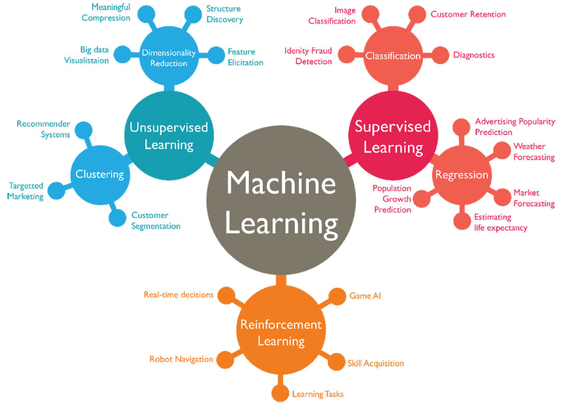
- Machine learning (ML) is the scientific study of algorithms and statistical models that computer systems use to perform a specific task without using explicit instructions, relying on patterns and inference instead.
- It is seen as a subset of artificial intelligence.
- Machine learning algorithms build a mathematical model based on sample data, known as "training data", in order to make predictions or decisions without being explicitly programmed to perform the task.
Content
- Why Machine Learning?
- Problems Machine Learning Can Solve
- Knowing Your Task and Knowing Your Data
- Essential Libraries and Tools
- scikit-learn
- Jupyter Notebook
- NumPy
- SciPy
- matplotlib
- pandas
- Python
- Why Python?
- A First Application: Classifying Iris Species
- Meet the Data
- Measuring Success: Training and Testing Data
- First Things First: Look at Your Data
- Building Your First Model: k-Nearest Neighbors
- Making Predictions
- Evaluating the Model Summary and Outlook
1. Why Machine Learning?
Two major disadvantages of hardcode rules:
The logic required to make a decision is specific to a single domain and task. Changing the task even slightly might require a rewrite of the whole system.
Designing rules requires a deep understanding of how a decision should be made by a human expert.
For machine learning, we just need using data to create the rules for our system. Change or add new data => retrain model => update the rules
2. Problems Machine Learning Can Solve

- Supervised learning: Machine learning algorithms that learn from input/output pairs (output has labelled)
- Unsuperviesd learning: only the input data is known, and no known output data is given to the algorithm.
2.1 Represent your data:
In a data tables including
- Each data point that you want to reason about (each email, each customer, each transaction) is a row
- Each entity or row here is known as a sample (or data point)
- Each property that describes that data point (say, the age of a customer or the amount or location of a transaction) is a column.
The columns—the properties that describe these entities are called features.

2.2 Knowing Your Task and Knowing Your Data
- Understanding the data
- How it relates to the task
First thinking about the problems:
- What question(s) am I trying to answer? Do I think the data collected can answer that question?
- What is the best way to phrase my question(s) as a machine learning problem?
- Have I collected enough data to represent the problem I want to solve?
- What features of the data did I extract, and will these enable the right predictions?
- How will I measure success in my application?
- How will the machine learning solution interact with other parts of my research or business product?
3. Essential Libraries and Tools
scikit-learn
- scikit-learn is an open source project, meaning that it is free to use and distribute, and anyone can easily obtain the source code to see what is going on behind the scenes.
Jupyter Notebook
- The Jupyter Notebook is an interactive environment for running code in the browser.
- A great tool for exploratory data analysis and is widely used by data scientists.
NumPy
- Contains functionality for multidimensional arrays, high-level mathematical functions such as linear algebra operations and the Fourier transform, and pseudorandom number generators.
import numpy as np

x = np.array([[1, 2, 3], [4, 5, 6]])
print("x:\n{}".format(x))
SciPy
- Provides,among other functionality, advanced linear algebra routines, mathematical function optimization, signal processing, special mathematical functions, and statistical distributions
from scipy import sparse

# Create a 2D NumPy array with a diagonal of ones, and zeros everywhere else
eye = np.eye(4)
print("NumPy array:\n", eye)
# Convert the NumPy array to a SciPy sparse matrix in CSR format
# Only the nonzero entries are stored
sparse_matrix = sparse.csr_matrix(eye)
print("\nSciPy sparse CSR matrix:\n", sparse_matrix)
data = np.ones(4)
row_indices = np.arange(4)
col_indices = np.arange(4)
eye_coo = sparse.coo_matrix((data, (row_indices, col_indices)))
print("COO representation:\n", eye_coo)
matplotlib
- visualizations
%matplotlib inline
import matplotlib.pyplot as plt

# Generate a sequence of numbers from -10 to 10 with 100 steps in between
x = np.linspace(-10, 10, 100)
# Create a second array using sine
y = np.sin(x)
# The plot function makes a line chart of one array against another
plt.plot(x, y, marker="x")
pandas
- Data wrangling and analysis
import pandas as pd

# create a simple dataset of people
data = {'Name': ["John", "Anna", "Peter", "Linda"],
        'Location' : ["New York", "Paris", "Berlin", "London"],
        'Age' : [24, 13, 53, 33]
       }

data_pandas = pd.DataFrame(data)
# IPython.display allows "pretty printing" of dataframes
# in the Jupyter notebook
display(data_pandas)
# Select all rows that have an age column greater than 30
display(data_pandas[data_pandas.Age > 30])
4. Python
Why Python?
Python has become the general programming language for many data science applications.
- It combines the power of general-purpose programming languages with the ease of use of domain-specific scripting languages like MATLAB or R.
- Python has libraries for data loading, visualization, statistics, natural language processing, image processing, and more.
Versions Used
import sys
print("Python version:", sys.version)

import pandas as pd
print("pandas version:", pd.__version__)

import matplotlib
print("matplotlib version:", matplotlib.__version__)

import numpy as np
print("NumPy version:", np.__version__)

import scipy as sp
print("SciPy version:", sp.__version__)

import IPython
print("IPython version:", IPython.__version__)

import sklearn
print("scikit-learn version:", sklearn.__version__)
# !pip install mglearn
5. A First Application: Classifying Iris Species

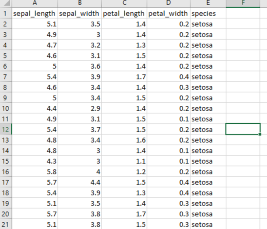
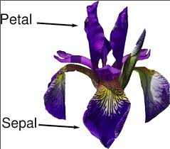
Iris data is a data sheet describing iris flowers, some measurements associated with each iris: the length and width of the petals and the length and width of the sepals, all measured in centimeters
5.1 Meet the Data
from sklearn.datasets import load_iris
iris_dataset = load_iris()
print("Keys of iris_dataset:\n", iris_dataset.keys())
The value of the key DESCR is a short description of the dataset.
print(iris_dataset['DESCR'][:193] + "\n...")
print("Target names:", iris_dataset['target_names'])
print("Feature names:\n", iris_dataset['feature_names'])
print("Type of data:", type(iris_dataset['data']))
print("Shape of data:", iris_dataset['data'].shape)
- The array contains measurements for 150 different flowers. Remember that the individual items are called samples (150) and their properties are called features (4)
print("First five rows of data:\n", iris_dataset['data'][:5])
print("Type of target:", type(iris_dataset['target']))
print("Shape of target:", iris_dataset['target'].shape)
print("Target:\n", iris_dataset['target'])
5.2 Measuring Success: Training and Testing Data
- We cannot use the data we used to build the model to evaluate it. Because our model can always simply remember the whole training set => predict the correct label for any point in the training set
- We should split the labeled data we have collected (here, our 150 flower measurements) into two parts:
- The training data: used to build our machine learning model, or training set.
- The test data: used to assess how well the model works; or test set, or hold-out set.
from sklearn.model_selection import train_test_split
X_train, X_test, y_train, y_test = train_test_split(iris_dataset['data'], iris_dataset['target'], random_state=0)
- This function extracts 75% of the rows in the data as the training set, together with the corresponding labels for this data. The remaining 25% of the data, together with the remaining labels, is declared as the test set.
print("X_train shape:", X_train.shape)
print("y_train shape:", y_train.shape)
print("X_test shape:", X_test.shape)
print("y_test shape:", y_test.shape)
5.3 First Things First: Look at Your Data
# create dataframe from data in X_train
# label the columns using the strings in iris_dataset.feature_names
import mglearn
iris_dataframe = pd.DataFrame(X_train, columns=iris_dataset.feature_names)
# create a scatter matrix from the dataframe, color by y_train
pd.plotting.scatter_matrix(iris_dataframe, c=y_train, figsize=(15, 15),
                           marker='o', hist_kwds={'bins': 20}, s=60,
                           alpha=.8, cmap=mglearn.cm3)
- We can see that the three classes seem to be relatively well separated using the sepal and petal measurements. This means that a machine learning model will likely be able to learn to separate them.
5.4 Building Your First Model: k-Nearest Neighbors
- KNN finds the point in the training set that is closest to the new point. Then it assigns the label of this training point to the new data point.
from sklearn.neighbors import KNeighborsClassifier
knn = KNeighborsClassifier(n_neighbors=1)
knn.fit(X_train, y_train)
5.5 Making Predictions
X_new = np.array([[5, 2.9, 1, 0.2]])
print("X_new.shape:", X_new.shape)
To make a prediction, we call the predict method of the knn object
prediction = knn.predict(X_new)
print("Prediction:", prediction)
print("Predicted target name:",
       iris_dataset['target_names'][prediction])
5.6 Evaluating the Model
- We can make a prediction for each iris in the test data and compare it against its label (the known species). We can measure how well the model works by computing the accuracy, which is the fraction of flowers for which the right species was predicted:
y_pred = knn.predict(X_test)
print("Test set predictions:\n", y_pred)
print("Test set score: {:.2f}".format(np.mean(y_pred == y_test)))
print("Test set score: {:.2f}".format(knn.score(X_test, y_test)))
6. Summary and Outlook
X_train, X_test, y_train, y_test = train_test_split(
    iris_dataset['data'], iris_dataset['target'], random_state=0)

knn = KNeighborsClassifier(n_neighbors=1)
knn.fit(X_train, y_train)

print("Test set score: {:.2f}".format(knn.score(X_test, y_test)))
Keep in your mind in this chapter:
- Machine learning and its applications
- Supervised and unsupervised learning.
- Split our dataset into a training set, to build our model, and a test set, to evaluate.
- Makes predictions for a new data point.
Comments !